The Fixed Point Number Representation

The fixed point number representation and its arithmetic will be one of the important skill set of any DSP engineer. Today I gonna talk in brief about what is Fixed Point Representation and how to use it.

Introduction
Basically arithmetics or any numerical computations are done via CPU (aka ALU - Arithmetic Logic Unit). However for certain arithmetics involving floating numbers (numbers with decimal point) a more specialized hardware is required - called FPU (Floating Point Unit). This act as a kind of co-processor to handle floating computation. During a floating operation the CPU generates TRAP and schedules the operations to the FPU and receives the result back.

Almost all the desktops (or PCs) have in build FPUs to support the these kinds of operation. However in Embedded systems or DSPs, its rare to find one, because of the factors like cost, size etc.
So now, how to handle floating arithmetics? In most of the cases the chipset manufacturers (ARM, TI etc) provides routines to achieve the same. These are the software implementation to emulate the floating point operation. But still this won't be sufficient, especially because of the speed of such emulation could effect the overall system performance. Now this the point where Fixed Point numbers comes handy.

Before getting into fixed point numbers, generally on computers, any number esp integers are represented in 2's complement format. That means any positive number will be represented in its binary format and negative number will be its 2's complement (one added to its complement).
The below table shows number and its 2's complement



This was the story of integers, the representation is bit different for floating points, on most of the modern computers they are represented in IEEE 754 standard [1]. However in fixed point representation we shall use 2's complement approach to represent a floating point number.

Welcome 'On-board'
Now lets dive into fixed point representation. Generally a floating number can be divided into two parts - a magnitude part and a fractional part. In fixed point representation we allocates sufficiently large number of bits to represent the number (to reduce the quantization error) for both magnitude and fractional part.
For example lets take 3.0 and analyze its binary values

As you can notice as we divide the decimal number by 2, the decimal point of the binary moves one point to the right, keeping the same binary representation and vice-versa. Decimal point shifts if we divide or multiply by 2 in binary or in case of decimal by 10.

Now lets talk about 'Q' format, where Q represents the number of Q format. Qf format gives the number of bits that are used to represent the fractional part. For example Q15 could be convey the meaning like 15 bits are used to represent the fractional part (out of 16 bit or 32 bit or more word length ). Here word length means the register size (like 8, 16, 32, 64 etc). Qm.f - where it represent both magnitude and fractional part, for example Q1.15 - 1 - magnitude bit and 15 fractional bits. Also the same could be used to show the sign bit as well.

The number of bits required to represent the fractional part depends upon the resolution/precision one wanted to achieve (incase of Single Precision floating representation one may need minimum 23 bits to represent the fractional part). For example with one bit we can have resolution of 0.5 (1/2^1). With 2 bits we can get resolution of 0.25 (i.e. 1/2^2) and so on. One should be careful while selecting the number of bits for fractional part to faithfully represent the number (with minimum rounding error). Thus to represent a fractional number you need to multiply by 2^x (where x denotes the number of bits - Qx). i.e, 0.142 in Q15 could be represented as 4653 in integer or 1001000101101 in binary representation. 

Now lets move on see how the effect of mathematical operation on Q format.In case of addition/subtraction of two Q format numbers the resultant Q format will be same  as of the addends (Qm + Qm = Qm+1). Addition and subtraction could be done with numbers of same Q format. Also one should take care of the overflow that can occur while addition.

Incase of multiplication Qm with Qn the resultant Q format shall be Qm+n. For division the resultant shall be Qm-n. As a last note its developers responsibility to keep track of the changes in the Q format in the code.

Next time we shall take an example filter and implement it floating point and then in fixed point to clearly understand the representation.

Till then keep Hac-King...

Also check this link for further research.

Soft Focus Effect using Gaussian Filter

Today lets try out some cool image processing stuffs. One of my favorite is soft focus.  Here I shall discuss how to achieve in an easy way using MATLAB or Octave. We will discuss the same using OpenCV some other day. So lets get started...

Soft focus gives an effect of spherical aberration by introducing a blur in the back ground. This creates an illusion that except the main object, rest all will be out of focus. Below I am giving a code snippet to achieve it on MATLAB.

function softFocus(iFile, iFocusRadii, oFile)
%softFocus Creates soft focus effect on an image.
%   iFile - Input image file name
%   iFocusRadii - Radius of focus area.
%   oFile - Output file name
%
%   This method uses Gaussian LPF approach and a
%   mask to create pin hole effect on the focus area.
%   This uses center as focus locaton however one
%   can easily change the logic to dynamically change
%   the focus point.
%   Ex: softFocus('Test.jpg', 50, 'Out.jpg')

if nargin < 3
    error('Insufficient number of input params');
end

close all

img = imread(iFile);

h = fspecial('gaussian',5, 10);
out = imfilter(img,h);

sz = size(img);
width = sz(2);
height = sz(1);
radius = iFocusRadii;   % area of focus
centerW = width/2;     % point where focus should fall
centerH = height/2;     % point where focus should fall

figure, imshow(img), title('Original Image');

[x,y]=ginput(2);

% create a mask for point hole effect
[W,H] = meshgrid(1:width,1:height);
mask = sqrt((W-x).^2 + (H-y).^2) < radius;

mask = uint8(mask * 255);

% create a smoothened border
h = fspecial('gaussian',50, 10);
mask = imfilter(mask,h);
mask = mask / 255;

% smoothening between focus and non-focus areas
% still better reduce the mask size and apply only
% iFocusRadii + 10 area to reduce amount of processing
for i = 1:height
    for j = 1: width

    alpha = mask(i, j);

 
    img1(i, j, :) = alpha * img(i, j, :) + (1 - alpha) * out(i, j, :);
 
    end
end

figure, imshow(img1), title('Soft Focused Image');

imwrite(img1, oFile);
end

Results:

The following images shows the effect of focus on fishes.

Input Image

Output Image

Below images shows a focus effect on kitten's face.

Input Image

Output Image

One could try out a lot of combinations to get better effects.

Next time we will discuss about more image effects. 

Till then keep Hac-King...

Sample Rate Converters

Sample Rate Converters (SRC) are used for changing the sampling rate (or frequency) of any signal. This include upsampling - increase the sampling rate or downsampling - the process of decreasing the sampling rate.

The upsampling process involves adding extra samples in between the existing samples (aka interpolation). A good example could be digital zoom in of an image. Downsampling on other hand is the process of removing samples (aka decimation), thus creating a signal with fewer samples, like zoom out of an image. My discussion here would narrow down on audio signal however similar approach could be used for images as well. I will discuss about SRC w.r.t images on some other day.
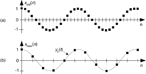
The below figure shows an original signal (a) and its downsampled version (b). The exact opposite is true for upsampling.

There are various applications of SRC in audio. A classical example could be conversion from audio on Compact Disc (44.1KHz) to Digital Audio Tape (48 KHz). Also it could be used while mixing multiple audio streams, or while rendering to a speaker which supports a different playback sampling rate, than the incoming audio. SRC usually a processor intensive algorithm and hence care must taken while choosing one.

Now lets discuss about various algorithms to achieve the same. Few of the approaches are:

1. By adding zeros in between samples and followed by a low pass filter to remove unwanted frequencies generated. For example to interpolate by L, one need to add L - 1 zeros between the samples. For decimation by M involves removing M - 1 samples in between. This method could also be used for fractional resampling as well (L = 1.0884 etc). Few optimization methods involves using polyphase FIR filters for filtering. For certain sampling rate, it could be a combination of L and M.

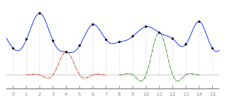
2. By windowed sinc interpolation method Band limited signals (sampled according to Nyquist criteria) . A good reference could be found in [1]. This makes use to sampling theorem for reconstructing an analog signal from a digital signal. Analog signal could be thought of signal with infinite interpolation. In this method a sinc function is interpolated depending upon minimum of source and target frequencies. This method is a trade-off between quality versus computation time. A detailed discussion will be followed with sample MATLAB code soon.

Few of the open source code available:

1. CCRMA - Bandlimited Interpolation.
2. Secret Rabbit Code - A GPL code for windowed sinc interpolation approach.
3. SSRC - A frequency domain approach.

One could find similar implementations SRC in various audio frameworks like SoX, Avisynth, ffmpeg etc.

As a last note, you can find a good comparisons tool for comparing between various open and commercially available SRCs here [2].


Next time we will be discussing more in-depth of bandlimited interpolation with a MATLAB source code. Till then keep Hac-king...